This is a new article reviewing a lot of old work but it also introduces some new theory and experimental results. For example: the idea that plant frequencies are equal in every direction is presented. This result came from calculations of velocity ratios at different angles in plants. Rotation of live wood samples in a vertical plane and the changes in output due to standing wave changes is included here.

Copyright ©2018 Wagner Research Laboratory

_________________________________________________________

Gravity responses and wave behavior in whole plants

Orvin E.Wagner

Wagner Research Laboratory

2902 Raywood Circle

Grants Pass, OR 97527

Summary

This paper presents data that lead to the conclusion that waves are a major factor in plant growth and that the waves interact with and are referenced to gravity. The observed waves behave somewhat like sound waves in resonant tubes with standing waves indicated by discretely spaced relatively wide charge locations on short blocks cut from live trees. Apparently plant internodal spacings are related to these charge spacings and analyses of thousands of plant-spacing measurements indicate that internode spacings do demonstrate wave involvement by their harmonic behavior. Electronic measurements confirm the wave frequencies. Angles that branches make with the horizontal or vertical appear to be predominately integral multiple of five degrees. The growth of reaction wood tends to confirm this effect. The data demonstrate that vertical wave velocities are generally greater than horizontal velocities by integral multiples of some basic velocity. The wave velocity seems to increase in steps from the horizontal to the vertical. This suggests that discrete charge locations move apart when a branch section is tipped from the horizontal to the vertical. Sinusoidal voltages from two probes on shielded live branch sections rotating in a vertical plane confirm this effect. Internodal spacings get larger on average, due to increasing wave velocity, as the angles that a branch makes with the horizontal increases in steps to the vertical. Fiber cells often get longer in a similar manner. Spacings converted to frequency and branch angles demonstrate wave behavior, and gravity interaction. The vertical to horizontal velocity ratios and the measurement of velocities indicate wave involvement related to gravity. The data confirming wave behavior connected with gravity appear to be unlimited. The waves demonstrated here might be some type of gravity waves, since they are obviously referenced to and otherwise tied to gravity.

Key words: cell lengths, gravity interactions, internodal spacings, standing waves in plants, velocity ratios.

___________________________________________________________

Introduction

Some details are understood on how a plant responds to gravity but it is still not well understood how whole plants respond to gravity (Salisbury 1993 and Fern, Wagstaff, and Digby 2000). For more than 25 years I have, as a physicist, have been making electrical measurements on plants. For about ten years I used probe pairs. After discovering waves in 1988, I used many probes often near a half wavelength apart. I measured many thousands of internodal spacings and angles of growth of trunks, branches, and their components. I found that plants of all measured species seem to be limited in the spacings and growth angles that are allowed, and these seem to repeat from plant to plant and species to species. There appear to be some very dominant spacings representing dominant frequencies as indicated by peaks on distributions. Actual measurement of frequencies on a spectrum analyzer indicated large amplitude signals for the dominant frequencies corresponding to the dominant spacings. Angles of growth appear to be mostly limited to integral multiples of about 5 degrees away from the horizontal in the species measured at least for the smaller angles. Horizontal spacings are usually the smallest on average but internodal spacing averages, (and often cell lengths) apparently increase in steps as the angle with the horizontal increases. The different velocities of waves in plants appear to control the latter behavior. The velocity of the waves apparently increases in steps thus increasing the spacings. This behavior suggests quantization. Quantization (in this case repetition of charge piles, incremental angles from the horizontal, a limited number of internodal spacings, or step changes in velocity) is often found in physics and my published data indicate that plants follow their own specialized quantization rules related to gravity. Quantization generally means that standing waves are involved. The waves discussed here seem to be governed by the rule for simple waves that velocity equals frequency times wavelength v=fλ.For example, obtaining a velocity and an internodal spacing (most often considered a half wavelength in this article) gives me two of the variables in the latter equation and so a frequency can then be calculated.

Waves are found everywhere. For example, all matter is largely made with standing quantum waves. Crystals are formed by standing waves (see physics texts). It is only natural that plants should utilize waves. Apparently, there is a set of many different frequencies of standing waves in plants with their corresponding half wavelengths. When the tip of a branch starts to grow at a bud in the spring, I assume it starts at a node and stops at an ending node, a half wavelength of a permitted frequency in the plant. The chosen permitted half wavelength is determined by the growing conditions. Internodal spacings are aptly named. When I first found wave in plants, I found charges piled at intervals along peeled tree trunks. These charge piles were wide and tapered off at the ends, as one would expect for standing waves (Fig. 1).

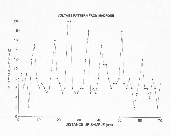Figure 1. Variation in voltage from a probe going up a Pacific Madrone sample quickly cut out from a longer sample. Not that the spacings are quite close to equal even though probe characteristics tend to cause errors. The results from this type of sample suggested to me that standing waves with shorter wavelengths than in the originating tree built up within a few minutes from cutting out the sample. A reference probe was placed in the bottom of the sample while a second probe was used to measure up the sample. This graph is from 1988 data used in Wagner 2001 and used by permission of Frontier Perspectives.

Regular intervals are observed only under the proper conditions because there are many frequencies in a plant represented by different spacings. I quickly cut sections out of the small trees, and it appeared that the charge concentration locations at least partially telescoped into the short sections. It was near 0^o Celsius when I did these first experiments. The low temperature may have helped eliminate some of the many frequencies and therefore spacings. I was thus often able to find simple resonant patterns. These waves might be special gravity waves since they seem to be so closely intertwined with gravity as will be pointed out later. I have been trying for years to reproduce and measure them in the laboratory with considerable success. In 1988, I called them W-waves because they were first found in wood. The experimental evidence indicates that they are longitudinal waves because branch spacings and thus half wavelengths are often much larger than very small trunk or stem diameters. Transverse waves need room for vibration perpendicular to the direction of travel.

Workers have been using probes in plants for many years. Much of the work was started by Bose (Bose 1907) and was continued by other workers such as Fensom (1964, 1985), Gensler (1974), Lund (1947), and Raber (1933). I used probes in plants for around 10 years before I stumbled onto the wave characteristics in 1988. I concluded that most of my early two-probe work was not revealing anything very important. One could relate some of the electrical curves obtained to plant characteristics but it appeared that much of the work was not repeatable (Wagner 1988 and Raber 1933). Not until multi-probing seemed to indicate wave characteristics did I become really excited. The later work and waves explained the non-repeatability of my early work. Much of the early work of others (e.g. Janick (1993)) appeared to be related to what were called action potentials, not of single cells as often defined but having to do with signals traveling along stems. Their work appears to be related to my measurements of wave velocities. I attempted to calculate the velocities of the signals involved in the Janick reference Figure 19-4 (Janick 1993) by methods I use in my work but the electrode spacings were not given. Otherwise the curves in the figure look like ones that I use in measuring wave velocities. My mearurements indicating standing waves don't appear to be directly related to action potentials.

Materials and Methods

Most of the data reported herein are from the following species: Grand fir (Abies grandis (Dougl.) Lindl), Douglas fir (Pseudotsuga menziesii (Mirb.) Franco), Red alder (Alnus rubra (Bong)), Big leaf maple (Acer macrophyllum Pursh.), Golden weeping willow (Salix sp. L.), False indigo (Amorpha fruiticosa), Delicious apple (Malus sp. Mill), Weeping birch (Betula sp. L.), Golden chinkapin (Castinopis chrsophylla (Dougl.) A. DC.), Ponderosa pine (Pinus ponderosa Laws), Hind's willow (Salix sp. L.), Incense cedar (Libocedrus decurrens Torr.), and Pacific madrone (Arbutus menziesii Pursh.). For electrical measurements, I used sharp top insulated steel probes (usually #2 steel pins) connected through high resistances (about ten megohms) to a high input impedance millivoltmeter. In the beginning a reference probe was placed in the bottom of the sample. In the initial work a second probe was quickly pushed in two millimeters or so, a reading recorded and then the probe was pulled out, and then pushed in farther along (usually up as in the plant) the sample and so on. Care was taken to prevent human body influences on the readings by using probes that were highly insulated from one's hands. Readings, when plant waves were discovered, were taken at about 0^o C in January 1988 (Wagner 1988). I quickly peeled the bark from the first samples. These peeled samples seemed to put out data for only about 25 minutes. Later I just removed the bark from the probed area when the readings didn't have to be taken so quickly or over a continuous area, such as for longer term measurements along a tree trunk. The spacing and angle measurements were taken using a centimeter rule and a #36 Polycast protractor (essentially a hanging weight with a scale; which can measure to about 0.25 degree). Angles were measured on branches of plants that were straight for at least four branch diameters. These straight portions were generally close to the trunk of a tree.

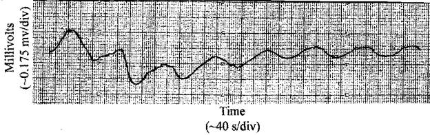
Velocities of waves in trees were measured by very fast wounding at one point on the plant and then recording and analyzing the resulting electrical signal from two probes placed as far apart as possible above the wounding point or farther out on a branch. The rise time (the initial straight line portion of a recorded curve) was considered the time the signal traveled between the two probes (Wagner 1996 and the Janick figure). Note that the rise time may appear longer than it should if the wounding pulse is not made fast enough.. The method used here has been checked many times using known distances and tree heights. One has to be careful about reflections from branches (Wagner 1988, 1996, & 2001). In the case of the sugar pine of Table 1, most of a small tree was brought into the lab and the vertical velocity was measured standing the tree upright and the horizontal velocity measured with the tree trunk level. Signal probes were two meters apart on the sugar pine and the measuring signal recorded on a strip chart recorder. Frequencies of the waves were measured on a Schlumberger 1201 spectrum analyzer (Wagner 1989, 1990-).

Measurements were taken from rotating 40 cm live samples (approx. 1 cm in diameter) in an aluminum box by taking bark off small areas near the ends to place probes (Fig 4). Leads from the probes carried the output through a plastic pipe that held and rotated the sample, to a strip chart recorder outside the aluminum box. The coaxial leads were made long enough so they could wind up on the plastic pipe as the pipe made one full rotation once every 16 minutes driven by a geared down motor. The leads were unwound for the next reading.

RESULTS AND DISCUSSION

Charge and Plant Spacings

In January 1988, I observed, using steel probes, that negative charge seemed to pile up at regular relatively large intervals, as indicated by probing, along quickly peeled small tree trunks. I then cut blocks out of small trees and quickly (within a minute) peeled and probed them. In this case, much closer spacings between charge piles were observed. The charged areas were wide as one would expect for standing waves.(Wagner 2001) (Fig. 1.) These areas developed within a few minutes (approx. 10 min) in the short blocks and then they quickly died out (within about 25 minutes) probably because these early samples were peeled. The charge spacings seemed to telescope after the blocks were cut out like sound wavelengths in a resonating sound tube when it is shortened. These shorter spacings apparently represent higher resonant frequencies (Wagner 1988, 2001). In 1988, I was first unaware that the blocks should have been of specific lengths, determined by the wavelengths of permitted dominant frequencies. This would have maximized the results due to resonance at a particular frequency, if the sample is an integral multiple of a half wavelength long. I probed so many samples that the effect finally became obvious even though with many samples the spacings weren't evenly spaced because more than one frequency was present. The low temperature at the time of the early measurements (near 0^o C) may have limited the observed frequencies and facilitated finding repeating spacings. I concluded that plant internodal spacings are related to the early negative charge spacing observations and are also quantized. The regular repeating spacings suggested standing waves. The waves seemed to be reflecting back and forth in the freshly cut samples building up a standing wave indicated by repeating charge piles observed within a few minutes from cutting. I assumed these charge piles were related to plant nodes. So the measurement of many thousands of internodal spacings began. I most often called these spacings half wavelengths of standing waves (Wagner 1990) with different spacings representing different frequencies in the plant. Actual measurement of frequencies of the waves confirm that the waves are real. I used a Sclumberger 1201 spectrum analyzer to measure frequencies for several years in the initial work to be sure that waves were being observed? (Wagner 1989, 1990). Actual measurements gave me the data so that I could label the frequency peaks in the published frequency distributions. I spent much of the time in my early work actually measuring frequencies of the waves. I observed larger amplitude signals at certain frequencies and their harmonics that seemed to be associated with the largest peaks (more spacings) found in distributions of plant spacings (Figs 2,3).

Note that the distributions are not smooth curves but show discrete peaks with apparently a limited number of frequencies. In the given figures the same velocity (96 cm/s) was used to calculate the frequencies from internodal spacings so the vertical and horizontal distributions appear to have different frequencies by a factor of 2 from a quick visual comparison of? Figures 2 and 3. Later work indicates that the apparent difference in frequencies is due to different velocities with the vertical velocities apparently greater than the horizontal by a factor of near 2 on average for the many species shown in these two distributions. The distributions and frequency measurements leave little doubt that waves are involved. Other measurements continue the proof (see all the Wagner references). Note that if a particular frequency actually had a higher velocity than 96 cm/s as was used in obtaining the two graphs shown it would appear as a higher frequency multiplied by an integral factor since velocities appear to be integral multiples of a basic velocity.

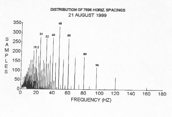
Figure 2. Includes data from internodal spacings on red alder, delicious apple, Himalaya blackberry (Rubus thyranthus), bracken fern (Pteridium aquilinium), golden chinkipin, weeping flowering cherry (prunus subhintella pendula ), Douglas fir, false indigo, big leaf maple, grand fir, ponderosa pine, weeping birch, Hind's willow, golden weeping willow, and Dutch elm (Ulmus hollandica). 96 cm/s was used to calculate the frequencies from spacings. The given frequencies and harmonics also appear on the spectrum analyzer used to measure and identify the frequencies. Near equal numbers of spacing were taken from each species.

Not only do live samples show the charge spacing effect but also samples soaked in saturated salt solution and partially dried develop similar, but much weaker (indicated by lower voltages from probing), charge piles (Wagner 1989). Note that ordinary porous materials don't show these charge spacings. There seems to be some electronic characteristics very special about the plant xylem structure that separates it from ordinary porous substances (Wagner and Deeds 1968). Studying salts in plant material first sparked my interest in studying live plant material. There is a whole list of special electrical characteristics that set it apart (mostly unpublished work). For example if one places steel probes near the ends of one of these samples and connects them to a high impedance voltmeter, one can often observe a change in the output voltage as one changes the sample orientation from upright to horizontal or vice versa. Also, if ac current is run through a salt filled wood sample the end that was 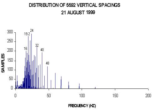lower in the tree heats up while the upper end remains cool (unpublished).

Figure 3. For this frequency distribution I used vertical spacings from prickly lettuce (Lactuca serriola), sweet corn (Zea mays saccarata), branch whorls from ponderosa pine, big leaf maple, delicious apple, red alder, weeping flowering cherry, golden chinkapin, Dutch elm, false indigo, Hind's willow, and weeping willow. I used 96 cm/s for the velocity to calculate the frequencies for comparison purposes. Actual velocities were often integral multiples of 96cm/s which would make many of the frequencies much higher using velocity equals frequency times wavelength. At the time the data were taken the larger velocities had not been measured. Spectrum analyzer data indicated frequencies of higher multiples were present.

Much of the same was found true for live samples where one removed a little bark to place the probes. The orientation effects can be attributed to charge location changes. The velocity for the waves apparently increases, due to increasing gravity, when one changes the sample orientation from horizontal to vertical, but the frequencies remain the same. The charge concentrations are farther apart because the wave velocity becomes larger. This suggests that the spacings between charge locations increase as the sample orientation is changed from horizontal to vertical. I slowly rotated several both live and salt filled samples in a vertical plane in a grounded aluminum box. A typical curve that resulted (for a 40 cm live sugar pine sample about 1 cm in diameter) is shown in Figure 4. This is another demonstration of wave behavior.

TABLE I. Results of measurements of vertical (V) and horizontal (H) branch and leaf spacings on trees. Also thousands of cell lengths from vertical and horizontal portions were measured and analyzed. Normally I took averages of the reciprocals of the spacings and cell lengths. When these averages are multiplied by a velocity they represent frequencies and one equates frequencies to find the velocity ratio. See the text. Vertical and horizontal velocities are being measured. Three sets are given here. Horizontal/vertical needles per unit length are given for sugar pine.

Consider incense cedar where it appears that the corresponding ratios for fibers indicate the shape of the tree. In other words, it appears that much higher frequencies (wavelengths of cell lengths instead of plant internode lengths) indicate the shape of the plant. On incense cedar, the branches often appear to be almost randomly placed, but the cell ratios seem to show the shape of the tree and a velocity ratio. Actual velocity measurements indicate the latter is the case. For incense cedar for the horizontal, I measured 369 cell lengths.At 45^o from the horizontal, I measured 336 lengths, and for the vertical 320 lengths. Note an apparent 5^o rule for fiber lengths. So in the case of incense cedar much higher frequencies (calling cell lengths half wavelengths) indicate the shape of the tree with v_vA_v=v₄₅A₄₅=v_hA_h (the frequencies are equal for every angle). The ratio derived from cell lengths v_v/v_h for incense cedar was 8/3 (actual from fiber lengths ratio 2.57). This compares favorably with the measured velocity ratio. See Table 1.

Another interesting tree is Pacific madrone. The branch spacings appear rather random and slope angles are hard to read because of the bumpiness of the tree surface. Here I measured fiber lengths from samples with growth angles of 0^o, 45^o, 65^o, and 80^o from the horizontal. The numbers of fibers measured were 342, 330, 367 and 341 respectively. The simple ratio v_v/v_h=9/5 (1.80 was the actual figure found) was found by extrapolation to the vertical using the 5^o rule with the equation v_hA_h=v₄₅A₄₅=v₆₅A₆₅=v₈₀A₈₀=v_vA_v.

The standard deviations for all the above averages ranged between 15 % and 45 % of the calculated averages. Many other trees and other plants were measured, but the above were chosen for typical examples of quantization with respect to the gravitational field. I made similar measurements on non-trees (e.g. prickly lettuce (Lactuca serriola L.) and sweet corn ) and obtained similar results. The internodal spacings are again quantized and apparently come from the general pool. These latter and other similar plants were not studied to the extent of the given trees and bushes reported in this article.

Another very simple possible approach to find velocity ratios on some trees like ponderosa pine is to analyze the most recent growth for the velocity ratio. For example, find the number of needles per unit length for vertical and horizontal from the top of a small Ponderosa pine tree and take the ratio of horizontal to vertical for a ratio of 3/1, or 2/1 for sugar pine.

When I first began my plant work, I was unaware that vertical velocities are usually larger than horizontal velocities and that there were multiple velocities. I used one initial measured velocity (96 cm/s which is still much faster than ionic diffusion velocities) for my initial calculations of frequency. I often graphed the number of spacings at all angles as the ordinate versus frequency as the abscissa. These graphs indicate that certain frequencies are predominant and that observed frequencies and thus certain spacings are predominant. The early graphs, however, still indicate the wave nature even though likely most of the frequencies were too low and should have been multiplied by integers like 2, 3, 4, 5, etc. The graphs still indicated that the frequencies are generally harmonics (integral multiples) of some lower basic frequency and that vertical and horizontal frequencies were similarly related. The early graphs indicate that frequencies (which were verified with a spectrum analyzer) and spacings repeat from species to species. Thus the wave nature of plants was proved at the start of the research (Wagner 1990, 1999a). I want to emphasize again that nutrition, temperature, and water available as well as other conditions determine a particular internodal spacing. There apparently is a limited pool of spacings from which the choice is made, however.

The wave velocity apparently increases slowly at first from the horizontal and rises more rapidly as the growth angle approaches the vertical. I found this from cell length data and other observations of plants. For example see Wagner (1999a), Table III, and correct for the 96 cm/s and use the idea that frequencies are equal at all angles.

Quantized Growth Angles

I measured angles that branches made with the horizontal and found them to be predominantly near multiples of five degrees from the horizontal or vertical thus finding that plant growth angles tend to be quantized (Wagner 1997, 1999a) with respect to the gravitational field. For example, angles with the horizontal were measured for branches on big leaf maple: 299 angles were measured. 198 angles were right on integral multiples of 5^o as best as could be measured with the protractor^. 53 angles were within 1 degree off from 5^o degree multiples. 48 angles were further off than 1^o from an integral multiple of 5^o. These results look very good due to the roughness of surfaces, disturbance of the branch on measurement, and other possible variables such as an angle that the plant has not corrected. If the angles were random the numbers would have been 62 at 5^o multiples, 118 angles would have been within one degree away from a multiple of 5^o, and 115 more than one degree away from a multiple of 5^o (zero is considered an angle here). Douglas fir provided 239 angles: the corresponding numbers are 114, 52, and 73 respectively (random 50, 95, 92). Red alder gave 335 angles with the numbers 232, 55,48 respectively (random 69, 132,129). Six other species around the laboratory provided 114 angles. The corresponding numbers are 80,22,12 respectively (random 24,45,44). From this kind of data it was concluded that growth angles tend to be quantized at integral multiples of 5o from the horizontal for many species at least for the smaller angles. The angles were distributed with more angles at the lower multiples of 5^o (See Wagner 1997, 1999a for plotted distributions). The results given here are typical examples. Tree branch angles both above and below the horizontal seem to be specified by the 5-degree rule discussed above. The 5^o quantized branch angles help explain the growth of reaction wood a tree grows to correct artificially changed branch angles (Salisbury and Ross 1985). This is also excellent evidence for the wave model.

DISCUSSION

A summary of some of the evidences that waves have much to do with plant operation is as follows:

(1) The placement of charge concentrations on the samples tested (Wagner 1988).

(2) Extensive measurement of plant frequencies with a low frequency spectrum analyzer. These measurements were both direct and by the use of beat frequencies where I applied a reference signal to the tree. (e.g.Wagner 1989, 1990.)

(3) The discrete organization of plant internode spacings as shown in Figures 2 and 3 for example.

(4) The behavior of plant internodal spacings growing in the presence of high voltage ac line electric fields. Some shorter plant internodal spacings seem to be nearly eliminated. It appears that the frequencies connected with these particular internodal spacings are close to line frequencies, which seems to prevent their growth is my hypotheses. The longer internode spacings appeared to become more dominant in the presence of the electric fields (Wagner 1995b, 2001).

(5) Measurement of the gravitational field within small holes in the xylem, using tiny accelerometers (and hanging weights in vertical holes in leaning trees) seemed to indicate a reduction in the gravitational field in vertical trunks of up to 25 % at near maximum sap flow. Also forces were measured in horizontal roots, which indicated assistance to sap flow. I attributed these forces initially to moving standing waves producing the forces. The gravity like forces measured apparently were just a small indication of the real gravity like forces involved because of the disturbance of the plant tissue in placing tiny measuring accelerometers. (Wagner 1991, 1995a) The brass shielding of the accelerometers and the distance of the accelerometer from the tree tissue indicated that the forces were gravity like and not Casimir or Van der Waals forces.

(6) The slope of branches at apparent predominant angles of integral multiples of 5^o (Wagner 1997).

(7) The sending of signals to surrounding trees indicating that the transmitting tree had been wounded (Wagner 1989)

It appears that there is a set of rules related to the gravitational field that constrain the plant. The described mechanisms may be all that is necessary to add to present theory to explain a plants response to gravity. Apparently, plant genotypes determine the velocities and velocity ratios while growing conditions predominantly determine the frequencies or spacings chosen from the available pool. Some special conditions apparently change the rules. It is likely that waves from different plants interact. For example, I found altered velocity ratios in shorter trees growing under taller trees where the sun provided nearly equal lighting to both trees. The vertical data seemed to lessen the velocity ratio to a lower value in the trees growing under taller ones (unpublished). There may be velocity ratios that are less than or equal to one and possibly different basic velocities than the ones given. Data indicate that velocities may be different during different seasons. Perhaps the wave velocity increases in steps from the horizontal to the vertical with each 5^o interval representing a step with spacings increasing accordingly. The given results together with previous findings then seem to indicate how whole trees and bushes respond to gravity. It appears that new growth, at the end of a branch, stops at the far node of a particular half wavelength (represented by a particular frequency and a velocity for that particular angle from the horizontal) determined by growing conditions. The data given here may imply that there may be an all-inclusive law, related to quantum mechanics, for plant growth that can be written as a simple equation or set of equations.

One of the best other evidences for the wave theory is the growth of reaction wood to correct a plant growth angle (Salisbury and Ross 1985) indicating that a plant part is "tuned" to a particular angle of growth. The averages derived from plant spacings and fiber lengths had large standard deviations (in the range of 15% to 45% of the averages obtained). The large standard deviations, where the spacing data is taken from several different plants to obtain a good sampling, and the simple velocity ratios that are, on average, within 1% of ratios of small integers constitutes mathematical proof that frequencies are the same at all angles and that the wave theory is correct. It reminds one of ordinary quantum mechanics where one takes averages to come up with exact characteristic quantities. Other proofs of the wave theory include actual measurement of the wave velocities and observing that the number of frequencies available to plants, although large, seem to be limited to specific values. These values seem to be harmonically related to one another (i.e. they seem to be integral multiples of more basic frequencies), which again indicates waves. See especially my earlier literature starting in 1988 for actual measured values of frequencies that indicate harmonic behavior. At first, I was unaware that velocities vary by integral multiples so the early published frequencies often need to be multiplied by 2 or 3 or 4 or maybe 5 or more and so on. The integral multiple and other wave characteristics are still evident, however. I did much more work than is indicated here. For example, as mentioned earlier, I measured relatively large gravity like forces associated with sap flow within xylem tissue (Wagner 1991, 1995a.). These forces tend to belie the usual theory of sap flow. I found that there seems to be a high energy density in xylem tissue associated with the waves in plants (Wagner 1993). I obtained up to 8 volts from polyethylene shielded silicon pn junctions placed in dark horizontal slits in trees. These might even be used as power sources with proper modification I also tried many approaches to these waves attempting to make them useful external to plants. For more details see the references, my web site, and other publications.

Note that the velocities of the observed plant waves both inside and outside of plants may suggest that some other than the commonly found wave medium is involved. I hypothesized that dark matter might be involved. Dark matter is everywhere and composes most of the mass of the universe. I wrote two documents using this hypothesis. Here I calculated that the wave velocities that I found in dark matter were comparable to the velocities that I found both inside and outside of plants (Wagner 1995 and Wagner 1999).

Acknowledgement: I thank my wife Claudia for reading the manuscript and making comments.

References

Bose, J.C. Comparative Electro-Physiology. Longman, Green, and Company 1907. pp. 1-760

Fensom, D.S. The bioelectric potentials of plants and their significance. Canad. J. Bot. 1964; 40:405-413.

Firn, RD, Wagstaff, C., and Digby, J. The use of mutants to probe models of Gravitropism.

J. of Experimental Botany 2000; 51(249):1323-1340.

Gensler, W. Bioelectric potentials and their relation to growth in higher plants.Ann. N.Y. Acad. Sci.1974; 238:280-299.

Janick, J. Horticultural Reviews, John Wiley and Sons, 1993. pp.411-414.

Lund, E.J. Bioelectric fields and growth. Univervsity of Texas Press 1947 pp. 1-391

Raber, O. Principles of Plant Physiology. The Macmillan Company. 1933. (extensive bibliography included).

Salisbury FB, Ross CW. Plant Physiology. Wadsworth, 1985 pp.370-71.

Salisbury FB, Gravitropism: Changing ideas. Horticultural reviews, John Wiley and Sons 1993. 15: 233-278..

Wagner OE. Wave behavior in plant tissue. N.W. Science 1988; 62:263-70.

Wagner OE. W-waves and plant communication. N.W. Science 1989; 63:119-128.

Wagner OE. W-waves and plant spacings. N.W. Science 1990; 64:28-38

.Wagner O.E. Acceleration changes within plants. Physiol. Chem. Phys NMR 1992; 24:29-34.

Wagner, O.E. Wave energy density in plants. Physiol. Chem. Phys. & Med. NMR 1993; 25:49-54.

Wagner OE Acceleration changes within living trees. Physiol. Chem. Phys. & Med. NMR 1995; 27:31-44.

Wagner OE. Waves in Dark Matter. Wagner Physics Publishing 1995 pp. 129-143

Wagner OE. Anisotropy of wave velocities in plants. Physiol. Chem. Phys. & Med. NMR 1996; 28:173-96.

Wagner OE. Quantization of plant growth angles with respect to gravity. Physiol. Chem. Phys. & Med. NMR 1997; 129: 63-69.

Wagner OE. A basis for a unified theory for plant growth and development. Physiol. Chem. Phys. & Med. NMR 1999; 31:109-29.

Wagner OE. Waves in dark matter. Physics Essays 1999; 12(1): 3-10.

Wagner OE. Structure in the vacuum. Frontier Perspectives 2001; 10(2): 23-34.

Wagner OE, Deeds WE. Some electronic properties of solutions in solid matrices.J. Phys. Chem. 1970; 74:288-298.

Plant Research | Main Page